Language models assign probability values to sequences of words. Those three words that appear right above your keyboard on your phone that try to predict the next word you’ll type are one of the uses of language modeling. In the case shown below, the language model is predicting that “from”, “on” and “it” have a high probability of being the next word in the given sentence. Internally, for each word in its vocabulary, the language model computes the probability that it will be the next word, but the user only gets to see the top three most probable words.

Neural language models are a fundamental part of many systems that attempt to solve natural language processing tasks such as machine translation and speech recognition. Currently, all state of the art language models are neural networks.

The first part of this post presents a simple feedforward neural network that solves this task. In the second part of the post, we will improve the simple model by adding to it a recurrent neural network (RNN). The final part will discuss two recently proposed regularization techniques for improving RNN based language models.

A simple model

To begin we will build a simple model that given a single word taken from some sentence tries predicting the word following it.

We represent words using one-hot vectors: we decide on an arbitrary ordering of the words in the vocabulary and then represent the nth word as a vector of the size of the vocabulary (N), which is set to 0 everywhere except element n which is set to 1.

The model can be separated into two components:

• We start by encoding the input word. This is done by taking the one hot vector representing the input word (c in the diagram), and multiplying it by a matrix of size (N,200) which we call the input embedding (U). This multiplication results in a vector of size 200, which is also referred to as a word embedding. This embedding is a dense representation of the current input word. This representation is both of a much smaller size than the one-hot vector representing the same word, and also has some other interesting properties. For example, while the distance between every two words represented by a one-hot vectors is always the same, these dense representations have the property that words that are close in meaning will have representations that are close in the embedding space.

• The second component can be seen as a decoder. After the encoding step, we have a representation of the input word. We multiply it by a matrix of size (200,N), which we call the output embedding (V). The resulting vector of size N is then passed through the softmax function, normalizing its values into a probability distribution (meaning each one of the values is between 0 and 1, and their sum is 1). This distribution is denoted by p in the diagram above.

The decoder is a simple function that takes a representation of the input word and returns a distribution which represents the model’s predictions for the next word: the model assigns to each word the probability that it will be the next word in the sequence.

To train this model, we need pairs of input and target output words. For the (input, target-output) pairs we use the Penn Treebank dataset which contains around 40K sentences from news articles, and has a vocabulary of exactly 10,000 words. To generate word pairs for the model to learn from, we will just take every pair of neighboring words from the text and use the first one as the input word and the second one as the target output word. So for example for the sentence “The cat is on the mat” we will extract the following word pairs for training: (The, cat), (cat, is), (is, on), and so on.

We use stochastic gradient descent to update the model during training, and the loss used is the cross-entropy loss. Intuitively, this loss measures the distance between the output distribution predicted by the model and the target distribution for each pair of training words. The target distribution for each pair is a one-hot vector representing the target word.

The metric used for reporting the performance of a language model is its perplexity on the test set. It is defined as \(e^{-\frac{1}{N}\sum_{i=1}^{N} \ln p_{\text{target}_i}}\), where \(p_{\text{target}_i}\) is the probability given by the model to the ith target word. Perplexity is a decreasing function of the average log probability that the model assigns to each target word. We want to maximize the probability that we give to each target word, which means that we want to minimize the perplexity (the optimal perplexity is 1).

The perplexity for the simple model¹ is about 183 on the test set, which means that on average it assigns a probability of about \(0.005\) to the correct target word in each pair in the test set. It’s much better than a naive model which would assign an equal probability to each word (which would assign a probability of \(\frac {1} {N} = \frac {1} {10,000} = 0.0001\) to the correct word), but we can do much better.

Using RNNs to improve performance

The biggest problem with the simple model is that to predict the next word in the sentence, it only uses a single preceding word. If we could build a model that would remember even just a few of the preceding words there should be an improvement in its performance. To understand why adding memory helps, think of the following example: what words follow the word “drink”? You’d probably say that “coffee”, “beer” and “soda” have a high probably of following it. If I told you the word sequence was actually “Cows drink”, then you would completely change your answer.

We can add memory to our model by augmenting it with a recurrent neural network (RNN), as shown below.

This model is similar to the simple one, just that after encoding the current input word we feed the resulting representation (of size 200) into a two layer LSTM, which then outputs a vector also of size 200 (at every time step the LSTM also receives a vector representing its previous state- this is not shown in the diagram). Then, just like before, we use the decoder to convert this output vector into a vector of probability values. (LSTM is just a fancier RNN that is better at remembering the past. Its “API” is identical to the “API” of an RNN- the LSTM at each time step receives an input and its previous state, and uses those two inputs to compute an updated state and an output vector².)

Now we have a model that at each time step gets not only the current word representation, but also the state of the LSTM from the previous time step, and uses this to predict the next word. The state of the LSTM is a representation of the previously seen words (note that words that we saw recently have a much larger impact on this state than words we saw a while ago).

As expected, performance improves and the perplexity of this model on the test set is about 114. An implementation of this model³, along with a detailed explanation, is available in Tensorflow.

The importance of regularization

114 perplexity is good but we can still do much better. In this section I’ll present some recent advances that improve the performance of RNN based language models.

Dropout

We could try improving the network by increasing the size of the embeddings and LSTM layers (until now the size we used was 200), but soon enough this stops increasing the performance because the network overfits the training data (it uses its increased capacity to remember properties of the training set which leads to inferior generalization, i.e. performance on the unseen test set). One way to counter this, by regularizing the model, is to use dropout.

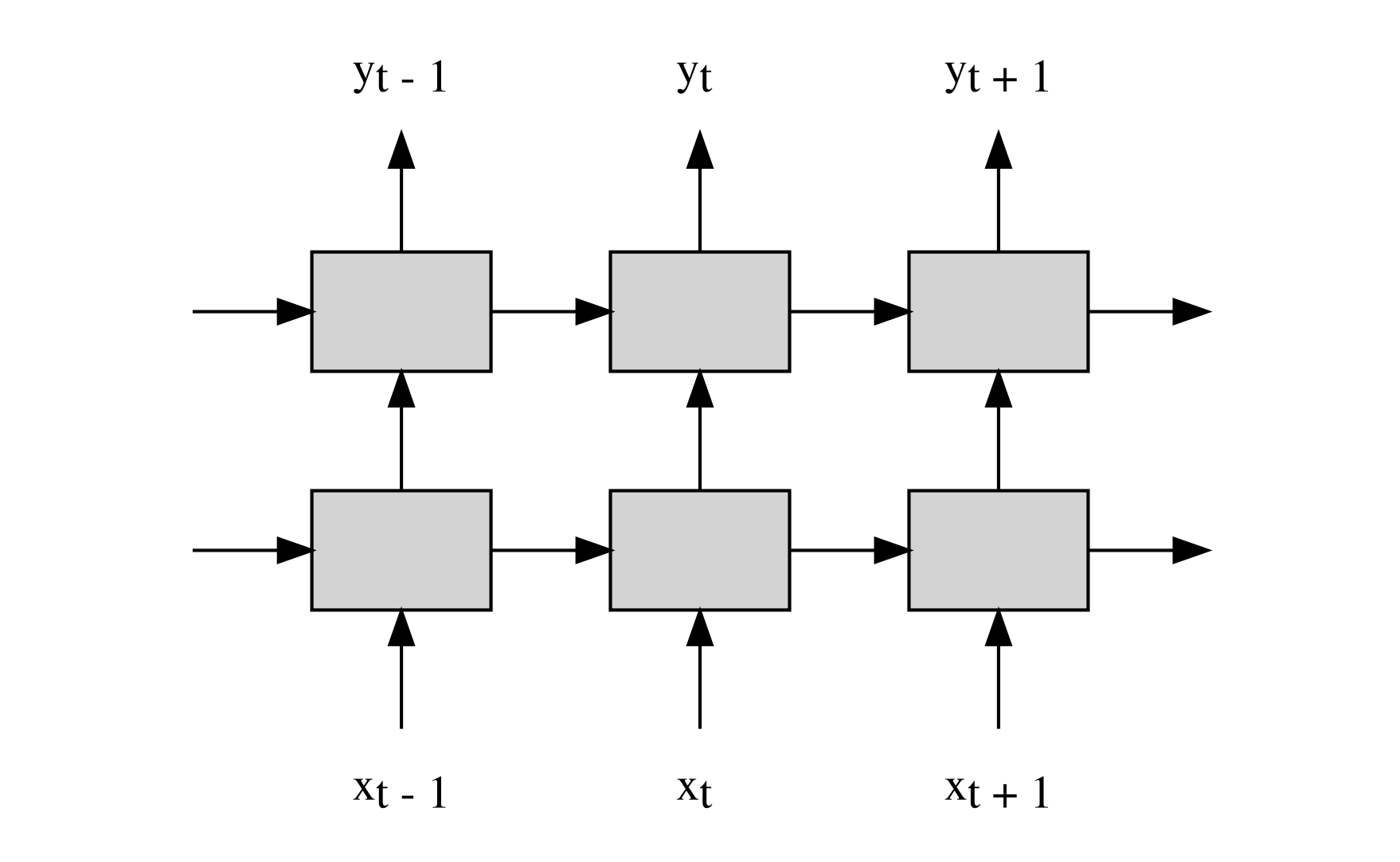
The diagram below is a visualization of the RNN based model unrolled across three time steps. x and y are the input and output sequences, and the gray boxes represent the LSTM layers. Vertical arrows represent an input to the layer that is from the same time step, and horizontal arrows represent connections that carry information from previous time steps.

We can apply dropout on the vertical (same time step) connections:

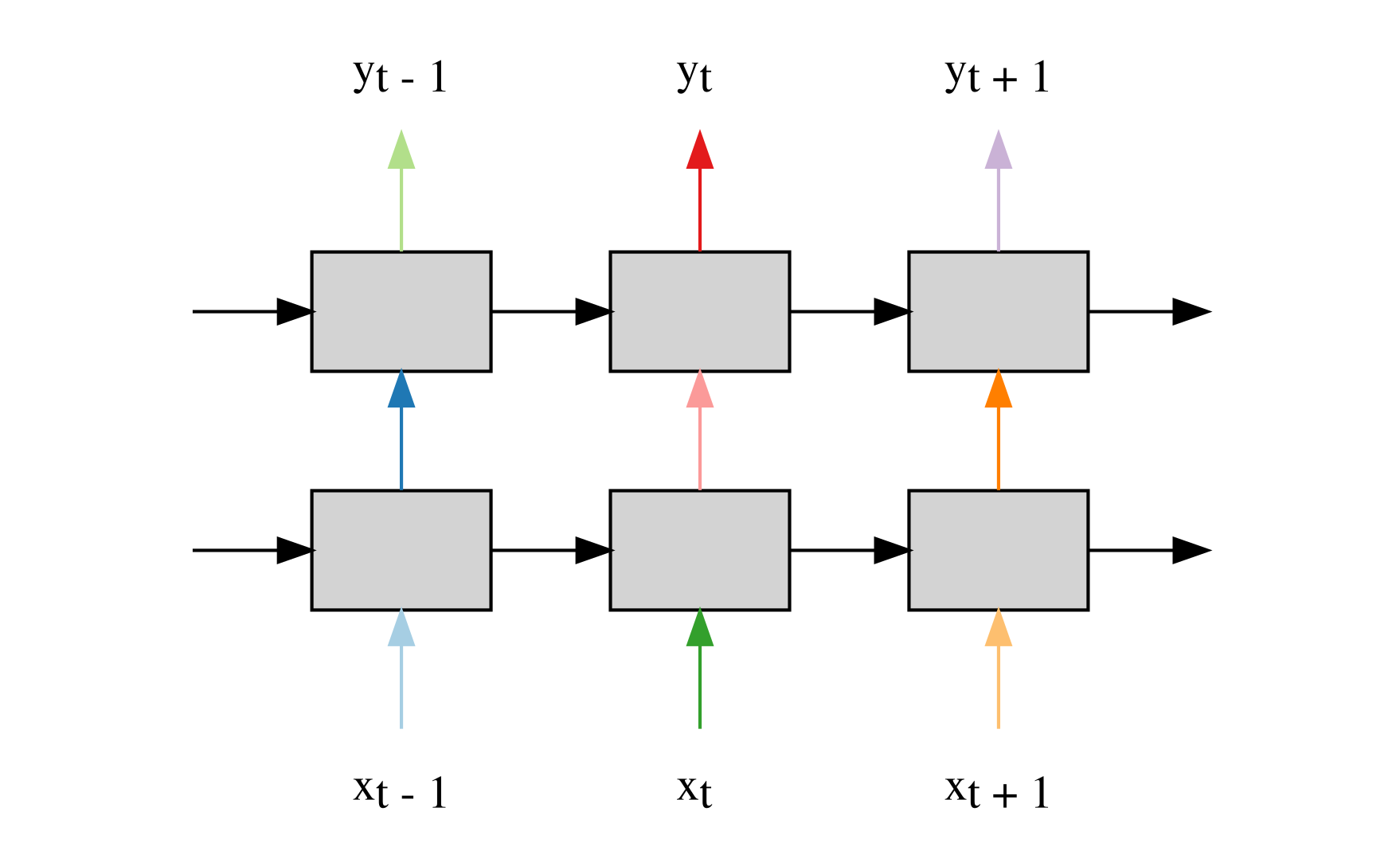
The arrows are colored in places where we apply dropout. A dropout mask for a certain layer indicates which of that layers activations are zeroed. In this case, we use different dropout masks for the different layers (this is indicated by the different colors in the diagram).

Applying dropout to the recurrent connections harms the performance, and so in this initial use of dropout we use it only on connections within the same time step. Using two LSTM layers, with each layer containing 1500 LSTM units, we achieve a perplexity of 78 (we dropout activations with a probability of 0.65)⁴.

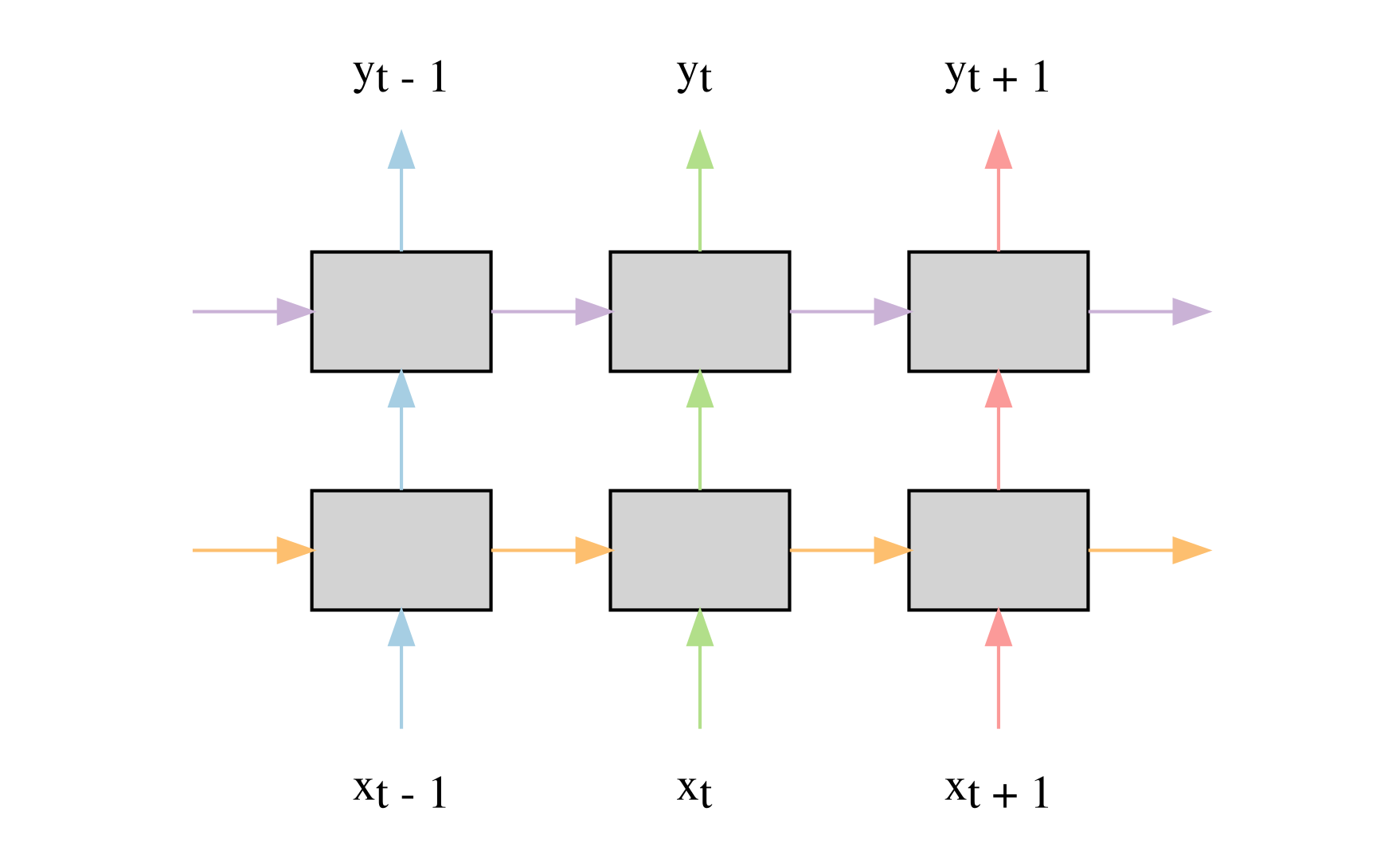
The recently introduced variational dropout solves this problem and improves the model’s performance even more (to 75 perplexity) by using the same dropout masks at each time step.

Weight Tying

The input embedding and output embedding have a few properties in common. The first property they share is that they are both of the same size (in our RNN model with dropout they are both of size (10000,1500)).

The second property that they share in common is a bit more subtle. In the input embedding, words that have similar meanings are represented by similar vectors (similar in terms of cosine similarity). This is because the model learns that it needs to react to similar words in a similar fashion (the words that follow the word “quick” are similar to the ones that follow the word “rapid”).

This also occurs in the output embedding. The output embedding receives a representation of the RNNs belief about the next output word (the output of the RNN) and has to transform it into a distribution. Given the representation from the RNN, the probability that the decoder assigns a word depends mostly on its representation in the output embedding (the probability is exactly the softmax normalized dot product of this representation and the output of the RNN).

Given the RNN output at a certain time step, the model would like to assign similar probability values to similar words. Therefore, similar words are represented by similar vectors in the output embedding. (Again, if a certain RNN output results in a high probability for the word “quick”, we expect that the probability for the word “rapid” will be high as well.)

These two similarities led us to recently propose a very simple method, weight tying, to lower the model’s parameters and improve its performance. We simply tie its input and output embedding (i.e. we set U=V, meaning that we now have a single embedding matrix that is used both as an input and output embedding). This reduces the perplexity of the RNN model that uses dropout to 73, and its size is reduced by more than 20%⁵.

Why does weight tying work?

The perplexity of the variational dropout RNN model on the test set is 75. The same model achieves 24 perplexity on the training set. So the model performs much better on the training set then it does on the test set. This means that it has started to remember certain patterns or sequences that occur only in the train set and do not help the model to generalize to unseen data. One of the ways to counter this overfitting is to reduce the model’s ability to ‘memorize’ by reducing its capacity (number of parameters). By applying weight tying, we remove a large number of parameters.

In addition to the regularizing effect of weight tying we presented another reason for the improved results. We showed that in untied language models the word representations in the output embedding are of much higher quality than the ones in the input embedding. This is shown using embedding evaluation benchmarks such as Simlex999. In a weight tied model, because the tied embedding’s parameter updates at each training iteration are very similar to the updates of the output embedding of the untied model, the tied embedding performs similarly to the output embedding of the untied model. So in the tied model, we use a single high quality embedding matrix in two places in the model. This contributes to the improved performance of the tied model⁶.

To summarize, this post presented how to improve a very simple feedforward neural network language model, by first adding an RNN, and then adding variational dropout and weight tying to it.

In recent months, we’ve seen further improvements to the state of the art in RNN language modeling. The current state of the art results are held by two recent papers by Melis et al. and Merity et al.. These models make use of most, if not all, of the methods shown above, and extend them by using better optimization techniques, new regularization methods, and by finding better hyperparameters for existing models.

---